Poisson distribution
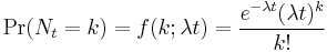
| Probability mass function The horizontal axis is the index k, the number of occurrences. The function is only defined at integer values of k. The connecting lines are only guides for the eye. |
|
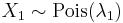
| Cumulative distribution function The horizontal axis is the index k, the number of occurrences. The CDF is discontinuous at the integers of k and flat everywhere else because a variable that is Poisson distributed only takes on integer values. |
|
| Notation |  |
|---|---|
| Parameters | λ > 0 (real) |
| Support | k ∈ { 0, 1, 2, 3, ... } |
| PMF |  |
| CDF |  for for  or or 
(where |
| Mean |  |
| Median |  |
| Mode |  |
| Variance | |
| Skewness |  |
| Ex. kurtosis |  |
| Entropy | ![\lambda[1\!-\!\log(\lambda)]\!%2B\!e^{-\lambda}\sum_{k=0}^\infty \frac{\lambda^k\log(k!)}{k!}](/2012-wikipedia_en_all_nopic_01_2012/I/b27b6cadba5878e13c577c34813aa485.png)
(for large |
| MGF |  |
| CF |  |
 is the
  is the
In probability theory and statistics, the Poisson distribution (pronounced [pwasɔ̃]) (or Poisson law of small numbers[1]) is a discrete probability distribution that expresses the probability of a given number of events occurring in a fixed interval of time and/or space if these events occur with a known average rate and independently of the time since the last event. (The Poisson distribution can also be used for the number of events in other specified intervals such as distance, area or volume.)
History
The distribution was first introduced by Siméon Denis Poisson (1781–1840) and published, together with his probability theory, in 1837 in his work Recherches sur la probabilité des jugements en matière criminelle et en matière civile (“Research on the Probability of Judgments in Criminal and Civil Matters”).[2] The work focused on certain random variables N that count, among other things, the number of discrete occurrences (sometimes called “arrivals”) that take place during a time-interval of given length.
The first practical application of this distribution was done by Ladislaus Bortkiewicz in 1898 when he was given the task to investigate the number of soldiers of the Prussian army killed accidentally by horse kick; this experiment introduced Poisson distribution to the field of reliability engineering.[3]
Applications
Applications of Poisson distribution can be found in every field related to counting:
- Electrical system example: telephone calls arriving in a system.
- Astronomy example: photons arriving at a telescope.
- Biology example: the number of mutations on a given strand of DNA.
The distribution equation
If the expected number of occurrences in a given interval is λ, then the probability that there are exactly k occurrences (k being a non-negative integer, k = 0, 1, 2, ...) is equal to
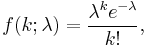
where
- e is the base of the natural logarithm (e = 2.71828...)
- k is the number of occurrences of an event — the probability of which is given by the function
- k! is the factorial of k
- λ is a positive real number, equal to the expected number of occurrences during the given interval. For instance, if the events occur on average 4 times per minute, and one is interested in the probability of an event occurring k times in a 10 minute interval, one would use a Poisson distribution as the model with λ = 10×4 = 40.
As a function of k, this is the probability mass function. The Poisson distribution can be derived as a limiting case of the binomial distribution.
The Poisson distribution can be applied to systems with a large number of possible events, each of which is rare. The Poisson distribution is sometimes called a Poissonian.
Poisson noise and characterizing small occurrences
The parameter λ is not only the mean number of occurrences ![E[k]](/2012-wikipedia_en_all_nopic_01_2012/I/b1cc7652a6e0109bca4a3b6161103019.png) , but also its variance
, but also its variance ![\sigma_k^2=E[k^2]-E[k]^2](/2012-wikipedia_en_all_nopic_01_2012/I/74f35e207faad026229be65ed734f65e.png) (see Table). Thus, the number of observed occurrences fluctuates about its mean λ with a standard deviation
(see Table). Thus, the number of observed occurrences fluctuates about its mean λ with a standard deviation  . These fluctuations are denoted as Poisson noise or (particularly in electronics) as shot noise.
The correlation of the mean and standard deviation in counting independent discrete occurrences is useful scientifically. By monitoring how the fluctuations vary with the mean signal, one can estimate the contribution of a single occurrence, even if that contribution is too small to be detected directly. For example, the charge e on an electron can be estimated by correlating the magnitude of an electric current with its shot noise. If N electrons pass a point in a given time t on the average, the mean current is  ; since the current fluctuations should be of the order
  (i.e., the standard deviation of the Poisson process), the charge
  can be estimated from the ratio
  . An everyday example is the graininess that appears as photographs are enlarged; the graininess is due to Poisson fluctuations in the number of reduced silver grains, not to the individual grains themselves. By correlating the graininess with the degree of enlargement, one can estimate the contribution of an individual grain (which is otherwise too small to be seen unaided). Many other molecular applications of Poisson noise have been developed, e.g., estimating the number density of receptor molecules in a cell membrane.
Related distributions
- If
 and
and  are independent, then the difference
  follows a Skellam distribution.
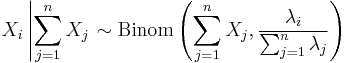
 - If and are independent, and
 , then the distribution of
  conditional on
  is a binomial. Specifically,
  . More generally, if X1, X2,..., Xn are independent Poisson random variables with parameters λ1, λ2,..., λn then
- The Poisson distribution can be derived as a limiting case to the binomial distribution as the number of trials goes to infinity and the expected number of successes remains fixed — see law of rare events below. Therefore it can be used as an approximation of the binomial distribution if n is sufficiently large and p is sufficiently small. There is a rule of thumb stating that the Poisson distribution is a good approximation of the binomial distribution if n is at least 20 and p is smaller than or equal to 0.05, and an excellent approximation if n ≥ 100 and np ≤ 10.[4]
- For sufficiently large values of λ, (say λ>1000), the normal distribution with mean λ and variance λ (standard deviation
 ), is an excellent approximation to the Poisson distribution. If λ is greater than about 10, then the normal distribution is a good approximation if an appropriate continuity correction is performed, i.e., P(X ≤ x), where (lower-case) x is a non-negative integer, is replaced by P(X ≤ x + 0.5).

- Variance-stabilizing transformation: When a variable is Poisson distributed, its square root is approximately normally distributed with expected value of about
 and variance of about 1/4.[5] Under this transformation, the convergence to normality is far faster than the untransformed variable. Other, slightly more complicated, variance stabilizing transformations are available,[6] one of which is Anscombe transform. See Data transformation (statistics) for more general uses of transformations.
 - If the number of arrivals in any given time interval
![[0,t]](/2012-wikipedia_en_all_nopic_01_2012/I/21b8fce671acf5fa4690193ad7ef3461.png) follows the Poisson distribution, with mean =
follows the Poisson distribution, with mean =  , then the lengths of the inter-arrival times follow the Exponential distribution, with mean
  .
.
Occurrence
The Poisson distribution arises in connection with Poisson processes. It applies to various phenomena of discrete properties (that is, those that may happen 0, 1, 2, 3, ... times during a given period of time or in a given area) whenever the probability of the phenomenon happening is constant in time or space. Examples of events that may be modelled as a Poisson distribution include:
- The number of soldiers killed by horse-kicks each year in each corps in the Prussian cavalry. This example was made famous by a book of Ladislaus Josephovich Bortkiewicz (1868–1931).
- The number of yeast cells used when brewing Guinness beer. This example was made famous by William Sealy Gosset (1876–1937).[7]
- The number of phone calls arriving at a call centre per minute.
- The number of goals in sports involving two competing teams.
- The number of deaths per year in a given age group.
- The number of jumps in a stock price in a given time interval.
- Under an assumption of homogeneity, the number of times a web server is accessed per minute.
- The number of mutations in a given stretch of DNA after a certain amount of radiation.
- The proportion of cells that will be infected at a given multiplicity of infection.
How does this distribution arise? — The law of rare events
In several of the above examples—such as, the number of mutations in a given sequence of DNA—the events being counted are actually the outcomes of discrete trials, and would more precisely be modelled using the binomial distribution, that is
In such cases n is very large and p is very small (and so the expectation np is of intermediate magnitude). Then the distribution may be approximated by the less cumbersome Poisson distribution
This is sometimes known as the law of rare events, since each of the n individual Bernoulli events rarely occurs. The name may be misleading because the total count of success events in a Poisson process need not be rare if the parameter np is not small. For example, the number of telephone calls to a busy switchboard in one hour follows a Poisson distribution with the events appearing frequent to the operator, but they are rare from the point of view of the average member of the population who is very unlikely to make a call to that switchboard in that hour.
Proof
We will prove that, for fixed  , if
, if

then for each fixed k
 .
.
To see the connection with the above discussion, for any Binomial random variable with large n and small p set  . Note that the expectation
  is fixed with respect to n.
First, recall from calculus
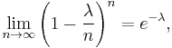
then since  in this case, we have
![\begin{align}
\lim_{n\to\infty} P(X_n=k)&=\lim_{n\to\infty}{n \choose k} p^k (1-p)^{n-k} \\
&=\lim_{n\to\infty}{n! \over (n-k)!k!} \left({\lambda \over n}\right)^k \left(1-{\lambda\over n}\right)^{n-k}\\
&=\lim_{n\to\infty}
\underbrace{\left[\frac{n!}{n^k\left(n-k\right)!}\right]}_{A_n}
\left(\frac{\lambda^k}{k!}\right)
\underbrace{\left(1-\frac{\lambda}{n}\right)^n}_{\to\exp\left(-\lambda\right)}
\underbrace{\left(1-\frac{\lambda}{n}\right)^{-k}}_{\to 1} \\
&= \left[ \lim_{n\to\infty} A_n \right] \left(\frac{\lambda^k}{k!}\right)\exp\left(-\lambda\right)
\end{align}](/2012-wikipedia_en_all_nopic_01_2012/I/4127ea0914f81678ca2b8ac4a3ef674c.png)
Next, note that
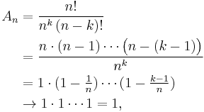
where we have taken the limit of each of the terms independently, which is permitted since there is a fixed number of terms with respect to n (there are k of them). Consequently, we have shown that
 .
.
Generalization
We have shown that if

where  , then
  in distribution. This holds in the more general situation that
  is any sequence such that
2-dimensional Poisson process
where
- e is the base of the natural logarithm (e = 2.71828...)
- k is the number of occurrences of an event - the probability of which is given by the function
- k! is the factorial of k
- D is the 2-dimensional region
- |D| is the area of the region
- N(D) is the number of points in the process in region D
Properties
- The expected value of a Poisson-distributed random variable is equal to λ and so is its variance. The higher moments of the Poisson distribution are Touchard polynomials in λ, whose coefficients have a combinatorial meaning. In fact, when the expected value of the Poisson distribution is 1, then Dobinski's formula says that the nth moment equals the number of partitions of a set of size n.
- The mode of a Poisson-distributed random variable with non-integer λ is equal to
 , which is the largest integer less than or equal to λ. This is also written as floor(λ). When λ is a positive integer, the modes are λ and λ − 1.
 - Given one event (or any number) the expected number of other events is independent so still λ. If reproductive success follows a Poisson distribution with expected number of offspring λ, then for a given individual the expected number of (half)siblings (per parent) is also λ. If fullsiblings are rare total expected sibs are 2λ.
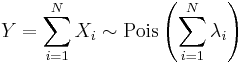
- Sums of Poisson-distributed random variables:
- If
 follow a Poisson distribution with parameter
  and
and  are independent, then
- also follows a Poisson distribution whose parameter is the sum of the component parameters. A converse is Raikov's theorem, which says that if the sum of two independent random variables is Poisson-distributed, then so is each of those two independent random variables.
- The sum of normalised square deviations is approximately distributed as chi-squared if the mean is of a moderate size (
 is suggested).[8] If
  are observations from independent Poisson distributions with means
  then
then 
- The moment-generating function of the Poisson distribution with expected value λ is
- All of the cumulants of the Poisson distribution are equal to the expected value λ. The nth factorial moment of the Poisson distribution is λn.
- The Poisson distributions are infinitely divisible probability distributions.
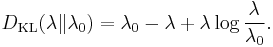
- The directed Kullback-Leibler divergence between Pois(λ) and Pois(λ0) is given by
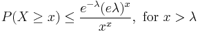
- Upper bound for the tail probability of a Poisson random variable
 .[9] The proof uses a Chernoff bound argument.
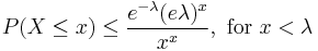
- Similarly,
Evaluating the Poisson distribution
Although the Poisson distribution is limited by
 ,
,
the numerator and denominator of  can reach extreme values for large values of
  or .
or .
If the Poisson distribution is evaluated on a computer with limited precision by first evaluating its numerator and denominator and then dividing the two, then a significant loss of precision may occur.
For example, with the common double precision a complete loss of precision occurs if  is evaluated in this manner.
A more robust evaluation method is:
Generating Poisson-distributed random variables
A simple algorithm to generate random Poisson-distributed numbers (pseudo-random number sampling) has been given by Knuth (see References below):
algorithm poisson random number (Knuth):
    init:
         Let L ← e−λ, k ← 0 and p ← 1.
    do:
         k ← k + 1.
         Generate uniform random number u in [0,1] and let p ← p × u.
    while p > L.
    return k − 1.
While simple, the complexity is linear in λ. There are many other algorithms to overcome this. Some are given in Ahrens & Dieter, see References below. Also, for large values of λ, there may be numerical stability issues because of the term e−λ. One solution for large values of λ is Rejection sampling, another is to use a Gaussian approximation to the Poisson.
Inverse transform sampling is simple and efficient for small values of λ, and requires only one uniform random number u per sample. Cumulative probabilities are examined in turn until one exceeds u.
Parameter estimation
Maximum likelihood
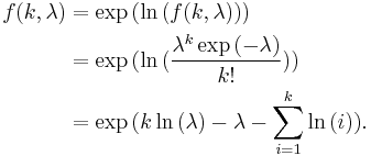
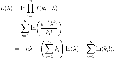
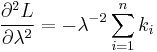
Given a sample of n measured values ki we wish to estimate the value of the parameter λ of the Poisson population from which the sample was drawn. To calculate the maximum likelihood value, we form the log-likelihood function
Take the derivative of L with respect to λ and equate it to zero:
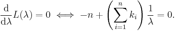
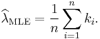
Solving for λ yields a stationary point, which if the second derivative is negative is the maximum-likelihood estimate of λ:
Checking the second derivative, it is found that it is negative for all λ and ki greater than zero, therefore this stationary point is indeed a maximum of the initial likelihood function:
Since each observation has expectation λ so does this sample mean. Therefore it is an unbiased estimator of λ. It is also an efficient estimator, i.e. its estimation variance achieves the Cramér–Rao lower bound (CRLB). Hence it is MVUE. Also it can be proved that the sample mean is complete and sufficient statistic for λ.
Bayesian inference
In Bayesian inference, the conjugate prior for the rate parameter λ of the Poisson distribution is the Gamma distribution. Let
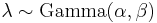
denote that λ is distributed according to the Gamma density g parameterized in terms of a shape parameter α and an inverse scale parameter β:
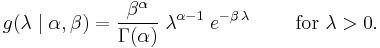
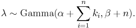
Then, given the same sample of n measured values ki as before, and a prior of Gamma(α, β), the posterior distribution is
The posterior mean E[λ] approaches the maximum likelihood estimate  in the limit as
  .
.
The posterior predictive distribution of additional data is a Gamma-Poisson (i.e. negative binomial) distribution.
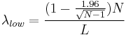
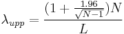
Confidence interval
A simple and rapid method to calculate an approximate confidence interval for the estimation of λ is proposed in Guerriero et al. (2009). This method provides a good approximation of the confidence interval limits, for samples containing at least 15 – 20 elements. Denoting by N the number of sampled points or events and by L the length of sample line (or the time interval), the upper and lower limits of the 95% confidence interval are given by:
The "law of small numbers"
The word law is sometimes used as a synonym of probability distribution, and convergence in law means convergence in distribution. Accordingly, the Poisson distribution is sometimes called the law of small numbers because it is the probability distribution of the number of occurrences of an event that happens rarely but has very many opportunities to happen. The Law of Small Numbers is a book by Ladislaus Bortkiewicz about the Poisson distribution, published in 1898. Some have suggested that the Poisson distribution should have been called the Bortkiewicz distribution.[10]
See also
- Coefficient of dispersion
- Compound Poisson distribution
- Conway–Maxwell–Poisson distribution
- Dobinski's formula
- Erlang distribution
- Incomplete gamma function
- Poisson process
- Poisson regression
- Poisson sampling
- Queueing theory
- Renewal theory
- Robbins lemma
- Skellam distribution
- Tweedie distributions
- Binomial distribution
- Negative binomial distribution
Notes
- ^ Gullberg, Jan (1997). Mathematics from the birth of numbers. New York: W. W. Norton. pp. 963–965. ISBN 039304002X.
- ^ S.D. Poisson, Probabilité des jugements en matière criminelle et en matière civile, précédées des règles générales du calcul des probabilitiés (Paris, France: Bachelier, 1837), page 206.
- ^ Ladislaus von Bortkiewicz, Das Gesetz der kleinen Zahlen [The law of small numbers] (Leipzig, Germany: B.G. Teubner, 1898). On page 1, Bortkiewicz presents the Poisson distribution. On pages 23-25, Bortkiewicz presents his famous analysis of "4. Beispiel: Die durch Schlag eines Pferdes im preussischen Heere Getöteten." (4. Example: Those killed in the Prussian army by a horse's kick.).
- ^ NIST/SEMATECH, '6.3.3.1. Counts Control Charts', e-Handbook of Statistical Methods, accessed 25 October 2006
- ^ McCullagh, Peter; Nelder, John (1989). Generalized Linear Models. London: Chapman and Hall. ISBN 0-412-31760-5. page 196 gives the approximation and the subsequent terms.
- ^ Johnson, N.L., Kotz, S., Kemp, A.W. (1993) Univariate Discrete distributions (2nd edition). Wiley. ISBN 0-471-54897-9, p163
- ^ Philip J. Boland. "A Biographical Glimpse of William Sealy Gosset". The American Statistician, Vol. 38, No. 3. (Aug., 1984), pp. 179-183.. http://wfsc.tamu.edu/faculty/tdewitt/biometry/Boland%20PJ%20(1984)%20American%20Statistician%2038%20179-183%20-%20A%20biographical%20glimpse%20of%20William%20Sealy%20Gosset.pdf. Retrieved 2011-06-22. "At the turn of the 19th century, Arthur Guinness, Son & Co. became interested in hiring scientists to analyze data concerned with various aspects of its brewing process. Gosset was to be one of the first of these scientists, and so it was that in 1899 he moved to Dublin to take up a job as a brewer at St. James' Gate... Student published 22 papers, the first of which was entitled "On the Error of Counting With a Haemacytometer" (Biometrika, 1907). In it, Student illustrated the practical use of the Poisson distribution in counting the number of yeast cells on a square of a haemacytometer. Up until just before World War II, Guinness would not allow its employees to publish under their own names, and hence Gosset chose to write under the pseudonym of "Student.""
- ^ Box, Hunter and Hunter. Statistics for experimenters. Wiley. p. 57.
- ^ Massimo Franceschetti and Olivier Dousse and David N. C. Tse and Patrick Thiran (2007). "Closing the Gap in the Capacity of Wireless Networks Via Percolation Theory". IEEE Transactions on Information Theory. http://circuit.ucsd.edu/~massimo/Journal/IEEE-TIT-Capacity.pdf.
- ^ Good, I. J. (1986). "Some statistical applications of Poisson's work". Statistical Science 1 (2): 157–180. doi:10.1214/ss/1177013690. JSTOR 2245435.
References
- Joachim H. Ahrens, Ulrich Dieter (1974). "Computer Methods for Sampling from Gamma, Beta, Poisson and Binomial Distributions". Computing 12 (3): 223–246. doi:10.1007/BF02293108.
- Joachim H. Ahrens, Ulrich Dieter (1982). "Computer Generation of Poisson Deviates". ACM Transactions on Mathematical Software 8 (2): 163–179. doi:10.1145/355993.355997.
- Ronald J. Evans, J. Boersma, N. M. Blachman, A. A. Jagers (1988). "The Entropy of a Poisson Distribution: Problem 87-6". SIAM Review 30 (2): 314–317. doi:10.1137/1030059.
- V. Guerriero, A. Iannace, S. Mazzoli, M. Parente, S. Vitale, M. Giorgioni (2009). "Quantifying uncertainties in multi-scale studies of fractured reservoir analogues: Implemented statistical analysis of scan line data from carbonate rocks". Journal of Structural Geology (Elsevier). doi:10.1016/j.jsg.2009.04.016.
- Donald E. Knuth (1969). Seminumerical Algorithms. The Art of Computer Programming, Volume 2. Addison Wesley.
External links
|
|||||||||||